
0. Summary
Rice Gene Index offers connections in Asian rice populations.
It establishs gene relationship between different accessions, based on de novo annotations and full-length transcripts. And it contains qualitative and quantitative information on transcriptomes across different accessions and tissues.
Some functions and tools are provided here, like Genes, Homologues, Collinearity, BLAST, JBrowse, GO enrichment and Gene Description.
How to search in RGI?
Search Gene ID, Gene Symbol, GO number, Swiss-Prot ID or biology description terms (Please search multiple elements in space intervals, like 'GO:0003677 MH63RS3');
Conversion familiar gene ID, like MSU7 and RAP-db, to other gene ID which are RGI provided by Homologues modules;
Input sequence to BLAST tool, and the alignment result could be used to other functions or tools.
0.1. AAA
RGI includes 16 accessions, 16 assemblies, and 18 annotations (IRGSP 1.0 genome of Nipponbare includes three annotations).
And we built name rules: accessions | assemblies | annotations, like "GOBOL SAIL | Os132424RS1 | Gramene(+IsoSeq)"
0.2. Gene annotations

With a set of unified de novo annotation performed by Gramene (unpublished) of the most of genomes, RGI further integrated the new genes and transcripts identified by newly sequenced Iso-Seq data into the annotation results.
The naming rules of de novo annotation: 'Os' + the accession name + '_' (or '.') + chromosome number + 'g' + seven place number, like OsIR64_01g0000270. (The annotated genes are ordered by gene location in chromosome and the seven place number is named in gene order which is at intervals of ten.)
The naming rules of genes from Iso-Seq data: similar to de novo annotation, except the seven place number which between intervals of ten of de novo annotation according to gene location order. The last number of the seven place number is from 1 to 9 and from A to Z if the gene number which inserted to the intervals of ten are greater than 9 (like OsIR64_01g0000271).
The Locus Tag Prefix were provided for each annotaion in "Accessions" page
Notably, RGI provided two types of common gene id ID (MSU7 and RAP-db) to help users search genes that they are interested in.
0.3. Description of homologous genes
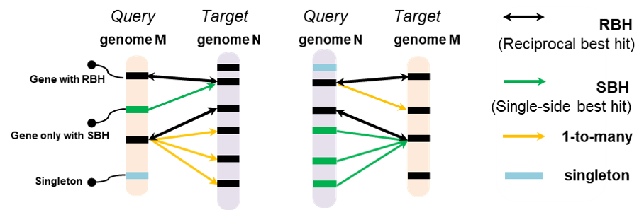
The GeneTribe is used to perform the homology inference, which combined sequence similarity and collinearity block information, and generated homology relationships including Reciprocal Best Hit (RBH), Single-side Best Hit (SBH), 1-to-many, and singleton. 1-to-1 is include RBH and SBH.
0.4. Ortholog gene indices
The rice genes are clusted to gene groups based on RBH relationships. The group of Ortholog gene indices direct relationships and indirect relationships between genes.
Nipponbare include 3 annotations (Gramene(+IsoSeq), MSU and RAP-db)
- Homolog group. Identified the RBH relationships between genes in accessions.
- Ortholog gene index. Clusted the homologs by connected graph methods. (The Ortholog gene index are named: 'OGI:' + chromosome number (The most frequent occurrence) + six place number (Using the order of genes in MH63 as a reference to determine the basic order of OGI, and for OGI not containing MH63 gene, query the position of MH63 gene in the OGI where its upstream gene is located, make insertion, and finally rearrange the order at intervals of 10.), likely OGI:12070020).
- OGI score. The score of OGI are 'C/D/S': + accession number in this OGI + / + all accession number , likely C:18/18.
- Prefix of the score: C: Core gene set, including all accession genes; D: dispensbale gene set, including partial accession genes; S: specific gene set, including genes specifically in accessions.
0.5. HomePage

1. Navbar, link to functions, tools and others
2. Search in RGI.
3. What's in RGI?
4. Ortholog Gene Index graph.
5. How to cite RGI?
6. The functions: Homologues, Gene Browse (GeneCard), Accessions, GenePair, MacroCollinearity and MicroCollinearity
7. The statistic of genomes and transcriptomes. The geneome table shows sample infomation of accessions which are RGI provided with the phylogentic tree
1. Homologues
1.1. Homologs table

1. Select assembly you want to search.
2. Input gene list by clipboard or file.
3. Select 1-to-1 or 1-to-many gene pairs.
4. Select other assemblies.
5. Run Homologous module.
6. Download the table of results to .csv file.
7. The results show the homologous gene IDs and homologous types (i.e. RBH and SBH). And the gene ID is link to GeneCard to show the comprehensive information.
8. 9. Show two sub-tools based on the results of homologous.
1.2. TreePlot & MSA

After run homologous table sub-module.
The TreePlot tool provides flexible options for building phylogenetic trees of different homolog groups. The main steps to using the new TreePlot tool are as follows:
1. Select the focused gene(s) from the gene list in the drop-down menu (step A). By default, homologs of all input genes will be used here. If users select part of the gene list, only the homologs of the selected genes will be analyzed.
2. Separate genes into different homologous groups (step B). By default, the tool will separate homologs of the input genes into different homologous groups. The tool first extracts homolog scores, calculated by GeneTribe (Chen et al., 2020), of all pairwise homologs from the MySQL database of RGI, and then uses the MCL algorithm (vanDongen, 2000) to group genes into different homologous groups. Each group will be analyzed separately. If this option is not checked, all genes will be analyzed together.
3. If users would like to separate homologs of all input genes into homologous group(s) (the default), they can skip the previous steps and click the GO button directly (Step C). A few seconds later, the output will appear in the bottom panel.
Result:

Figure Result
The output panel contains a table of homologous groups, an option to control which homologous group will be shown, multiple sequence alignments, and phylogenetic trees. The detailed descriptions of the output are as follows:
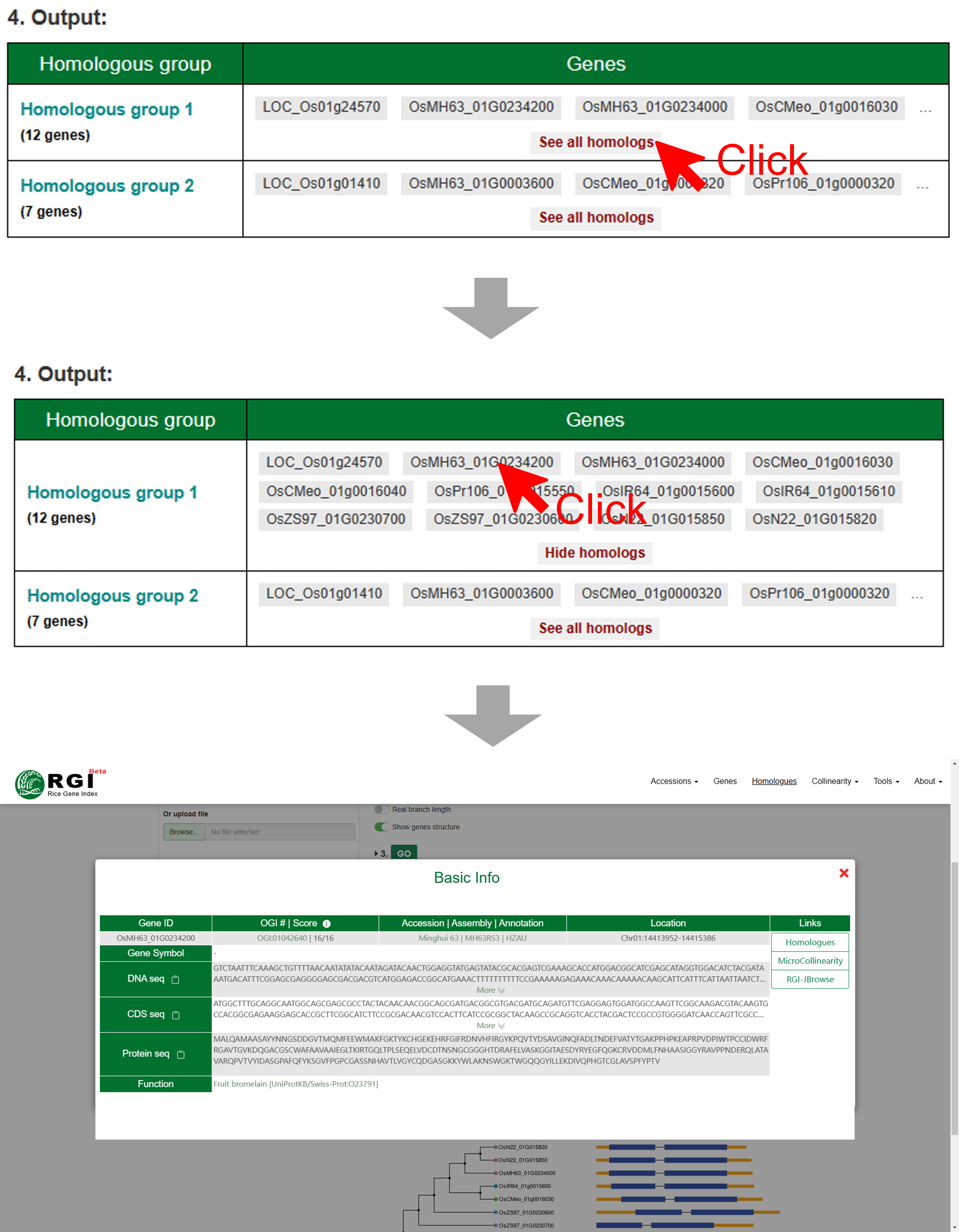
1. The homologous group table shows gene counts and gene IDs per homologous group (the output A in Figure Result). If users would like to view detailed information about genes in the homologous group, they can click the “See all homologs” button. All the genes will be shown in the cell of table. Furthermore, if users click one gene ID directly, a popup window will appear. The popup window shows the gene ID, symbol name, orthology, genome, annotation, location, sequence, function description, and quick links to other tools
2. Users can select one interested homologous group by clicking the drop-down menu “view homologous group” (the output B in Figure Result). The selected homologous group will be updated in real time at the bottom.
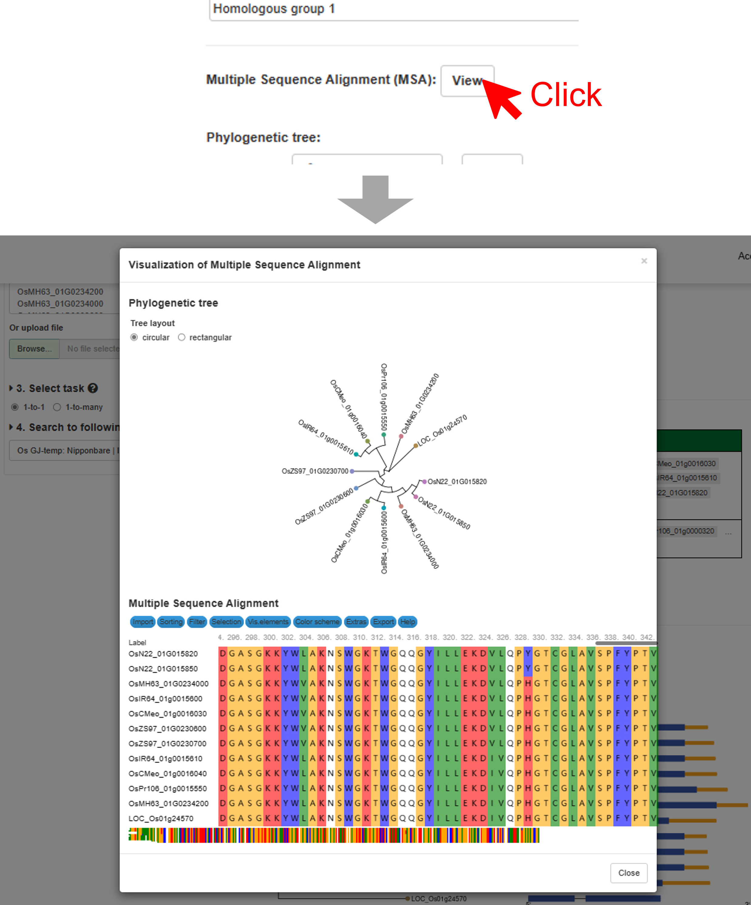
3. Users can click the “View” button (the output C in Figure Result) to view the detailed information about the multiple sequence alignment of the interested homologous group. A popup window containing the MSA of the interested homologous group will appear. MSA will be updated in real time according to the “view homologous group” menu.
4. The phylogenetic tree of one interested homologous group (the output D in Figure Result). The tree will be updated in real time according to the “view homologous group” menu.
1.3. GeneDis

After run homologous table sub-module.
1. Select assembly you want to show.
2. Choose whether to display gene IDs
3. Run GeneDis sub-module.
4. Download the image. User cloud choose figure format and size.
Result. Each gray bar represents a chromosome, gene colors are grouped by homologous gene sources, the horizontal scale indicates the size of the chromosomes.
2. Genes
2.1. GeneCard
GeneCard has multiple entries. The most convenient interface is to search for gene ID through the search box on the homepage, other entries are included in Homologues, Genepair, Microcollinearity, BLAST, JBrowse and GeneDescription.

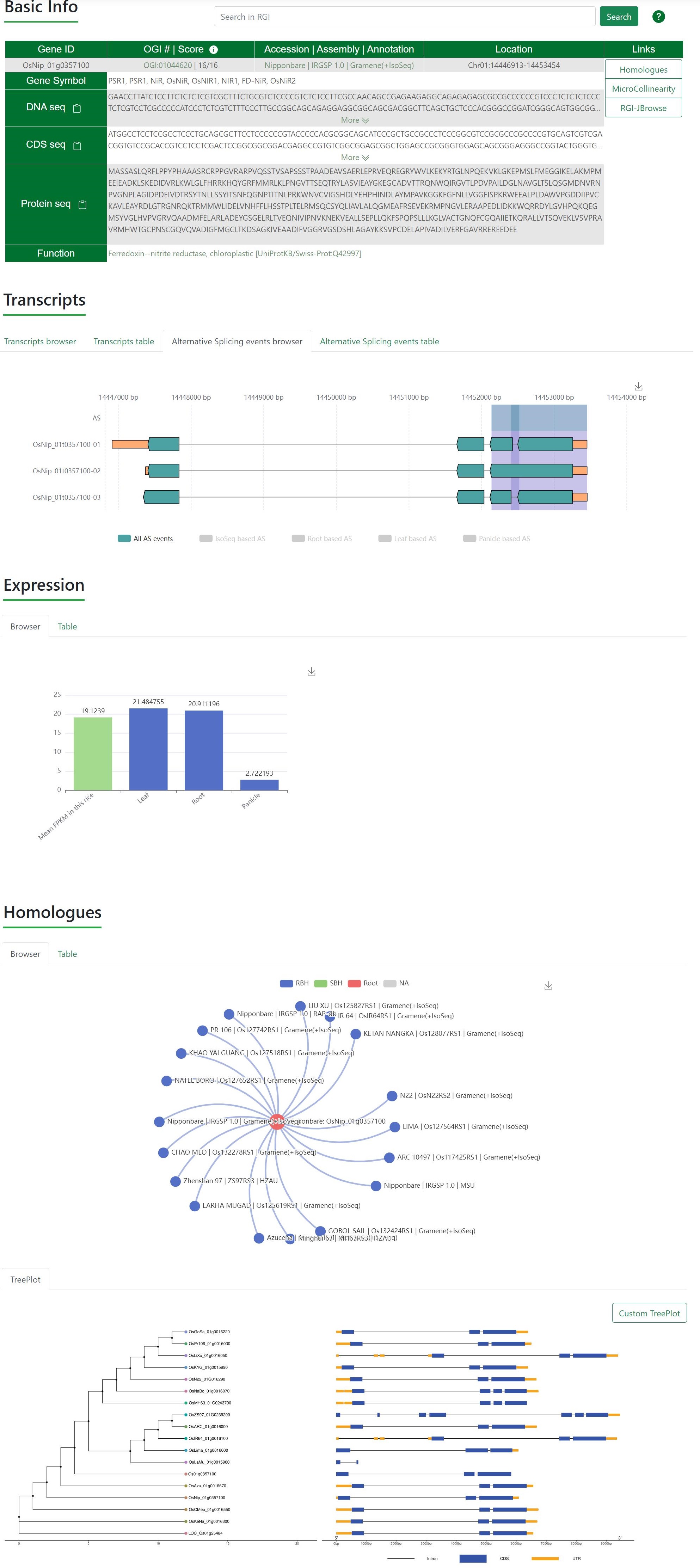
Basic Info. List the basic information such as gene ID, accession, location, gene sequence, CDS sequence, longest protein sequence and links for accessing Homologues, Microcollinearity and JBrowse (MSU and RAP-db links to Ricevarmap2 etc.).
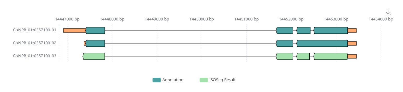
Transcripts. Visualize and list the structure of the transcripts. Users can visualize the interactive graphs by click labels which show the source of transcripts. The transcripts were derived to de novo annotations and Iso-Seq data (Annotation and ISOSeq Result). The graph could be downloaded by tap the icon in the top right.
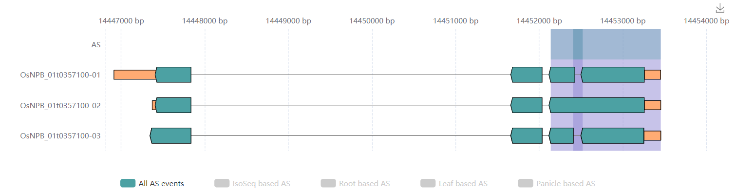
Transcripts.Alternative Splicing Events. Visualize and list the AS events. Users can visualize the interactive graphs by click labels which show the source of AS events. The AS events were derived to all AS events, Iso-Seq based AS events and AS events which involved transcripts are from leaf, root, or panicle. The graph could be downloaded by tap the icon in the top right.

Expression. Visualize and list the expression value (FPKM) of the gene in tissues (leaf, root and panicle).
Homologues. Visualize and list the homologs of this gene.

Homologues.TreePlot. tree and gene structures of these homologs.
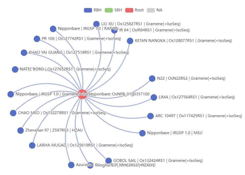
2.2. OGI graph

Users could enter the page from genecard and search directly related homologs and indirectly related genes.
3. Accessions
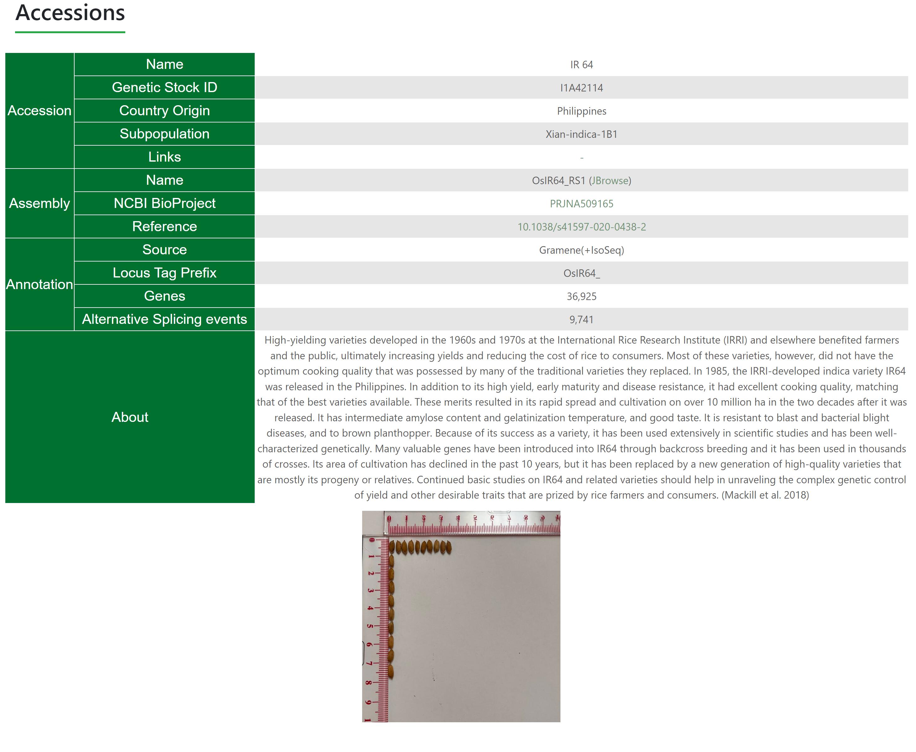
Accessions show the comprehensive information of rice accessions. It shows Accession name, NCBI BioProject, Genetic Stock ID, Country Origin, Subpopulation, Annotation, Gene number, AS events number, External Link, Description and Images.
4. Genepair
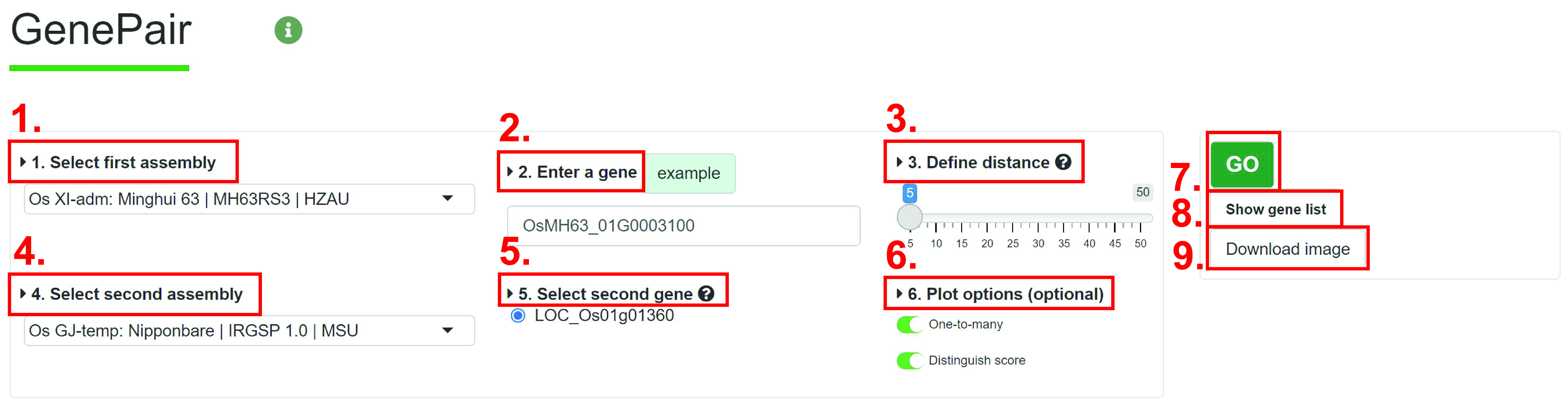
1. Select assembly you want to search.
2. Input gene ID you want to search.
3. Define a distance. The Distance is used to determine total number of genes on the chromosome, it refers to the number of flanking genes.
4. Select another assembly.
5. User will see multiple gene IDs, and user should select one.
6. (Optional) The optional options. One-to-many: All homologous genes will be showed, otherwise, only 1-to-1. Distinguish scores: Scores will be grouped by different line type.
7. Run Genepair module.
8. View location of genes in figure.
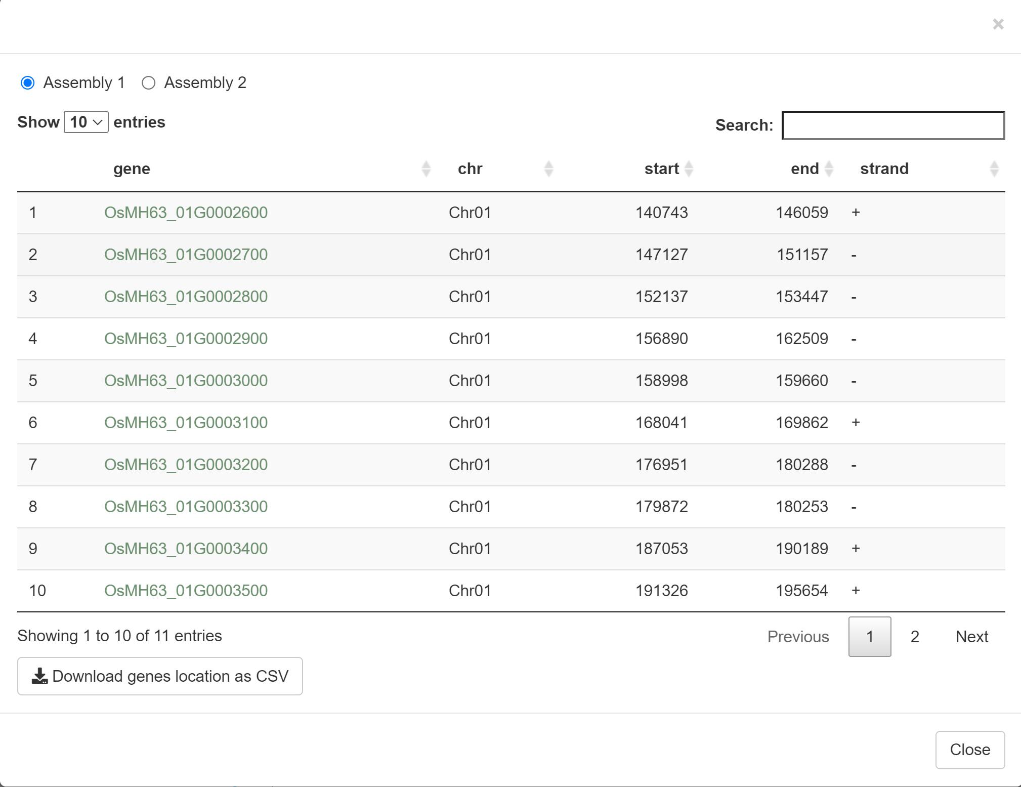
The output result includes gene ID, chromosome, start location, end location, and strand.
9. Download the image. User cloud choose figure format and size.
Result:

The output result contains two parts, which are the upper chromosome collinearity and the lower local collinearity.
The ‘Dot Plot’ panel visualize the macro-collinearity among all chromosomes. The collinearity blocks in the ‘Dot Plot’ are clickable, and the corresponding information may be displayed above the ‘Dot Plot’ box, which provides links to ‘JBrowse’. At the right panel, the colors of collinear block are grouped by Collinear Block Score (CBS). The higher the CBS, the better the collinearity. The lower chromosome corresponds to the first genome, and the upper chromosome corresponds to the second genome. The inputted gene is marked by red triangle.
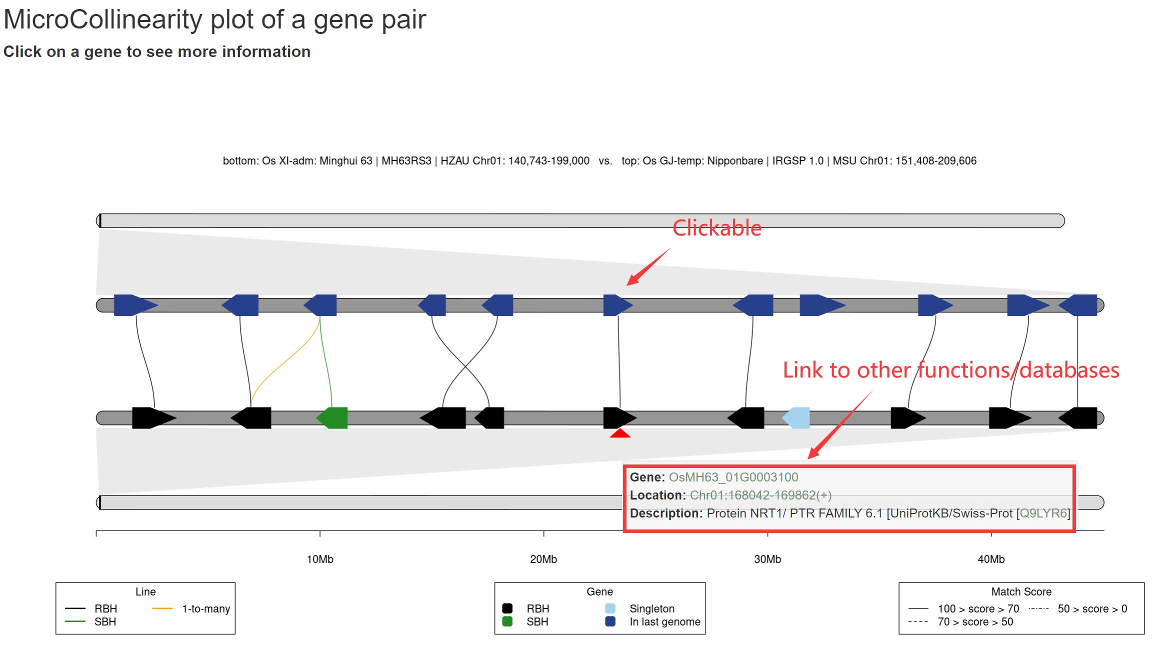
In the local collinearity, the genes and lines (i.e. homologous gene pairs) on the first chromosome region are grouped by homologous relationships (i.e. RBH, SBH, singleton, and 1-to-many). Color priority: RBH > SBH > 1-to-many. All homologous lines are grouped as three groups by score, which are 0-50, 50-70, and 70-100.
5. MacroCollinearity
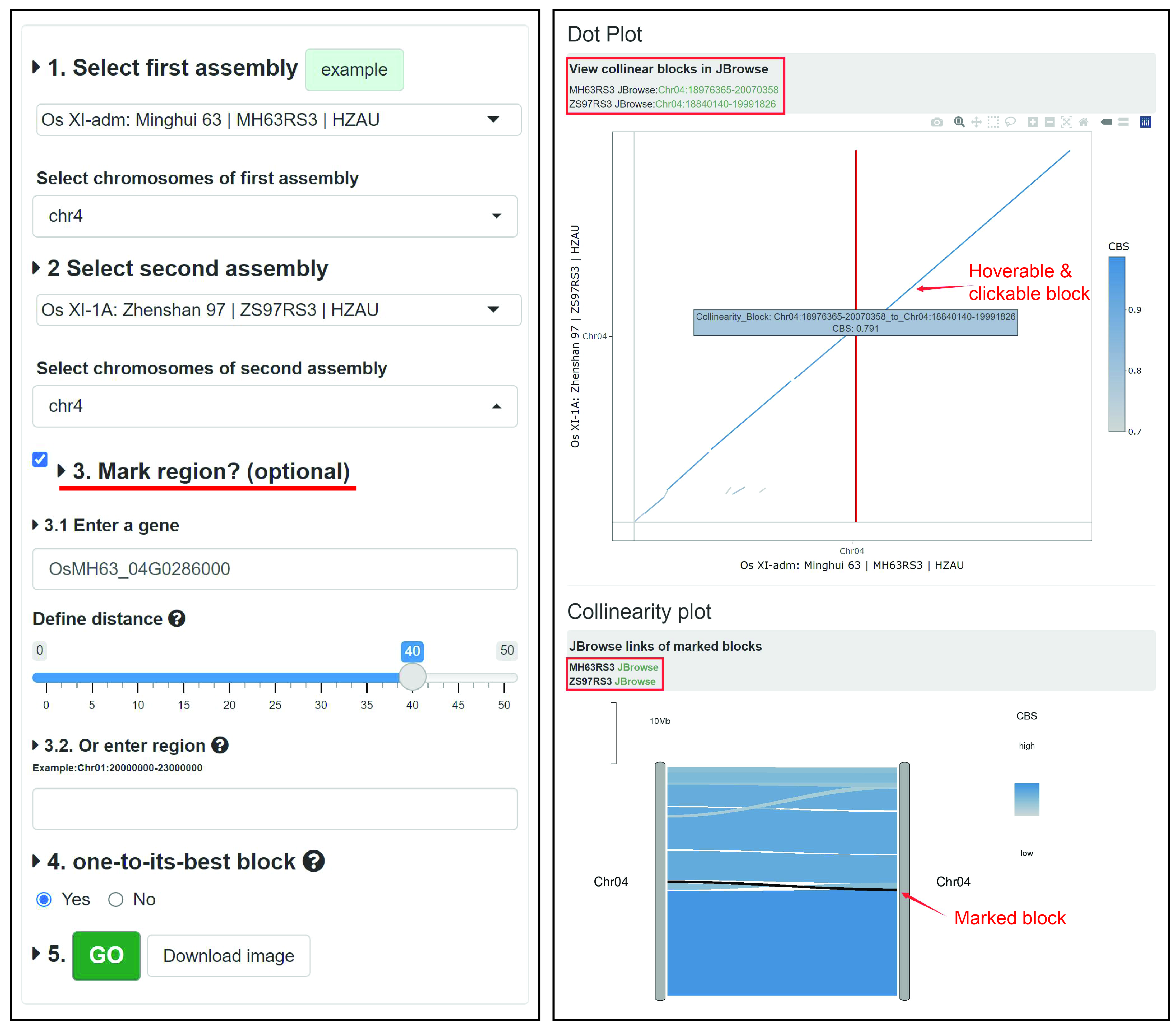
The 'MacroCollinearity' module provides chromosome-level collinearity analysis and visualization. Users can compare multiple chromosomes of two genomes and draw a collinearity plot and an interactive Dot Plot, and quickly view the corresponding region and the genes it contains through the link generated by the collinearity block in JBrowse.
Example: We compare chromosome 4 of Minghui 63 and Zhenshan 97, and choose to label (optional) the region contained by 40 genes on both sides of the gene OsMH63_04G0286000 (or choose to label by chromosome coordinates), and choose to show only the best collinearity block (Figure left). The results are shown on the right of Figure. In both 'Dot plot' and 'Collinearity plot', a large inversion variation on chromosome 4 was found in both genomes. In 'Dot plot', the red line is the starting position of the marked area, and the user can click on the collinear block in the figure to get a link to 'JBrowse' to quickly view the genes contained in the corresponding area. 'Dot plot' also supports operations such as zooming. In 'Collinearity plot', the black is the marked area, and users can quickly link to the marked area in 'JBrowse' (Figure right).
6. MicroCollinearity

The 'MicroCollinearity' module provides analysis and visualization of gene-level collinearity. This module can draw the homologous relationship diagram of the target gene and its flanking genes in a given genome. Users can trace the homologous (evolutionary) relationship based on the known phylogenetic tree, and click the gene ID to view the detailed information of the gene and link Go to the GeneCard page.
Example: We analyzed the homology relationship between OsMH63_01G0003100 in Minghui 63, IR 64 and Zhenshan 97 genes, and chose to display the 5 flanking genes of this gene, and selected to display 'one-to-many', 'Distinguish score' and 'Real gene spacing' (users can also freely adjust the display information and font color size). As shown in Figure, the results are sorted according to the known species tree, and the homologous relationship in other accessions is traced from the query gene (and flanking genes). The colors and styles of genes and lines represent different homology relationships. The gene node in the figure can be clicked to generate a pop-up window displaying basic information and linking to the 'GeneCard' page.
The genes and lines (i.e. homologous gene pairs) are grouped by homologous relationships (i.e. RBH, SBH, singleton, and 1-to-many). Color priority: RBH > SBH > 1-to-many. All homologous lines are grouped as three groups by score, which are 0-50, 50-70, and 70-100. The input gene is marked by red triangle. Only the genomes that have collinear block will be showed. You should trace evolutionary hsitory of genes from bottom to top. The left tree is pre-computed.
7. BLAST
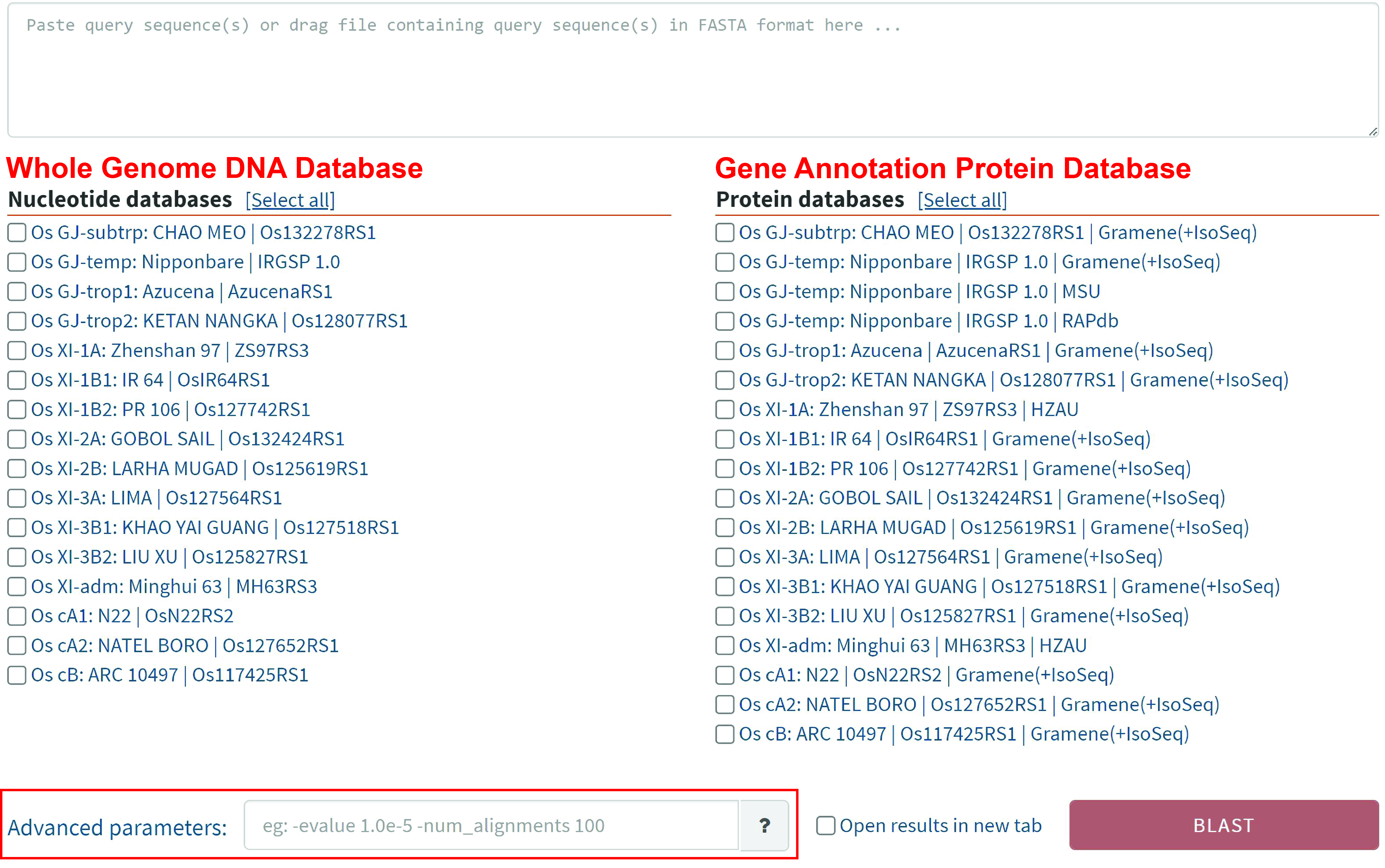
Users can start from DNA or protein sequences and use RGI's built-in BLAST tool to search in 16 genome sequence databases and 18 annotated gene protein databases. Users can customize the comparison according to the parameters in "?".
Result:
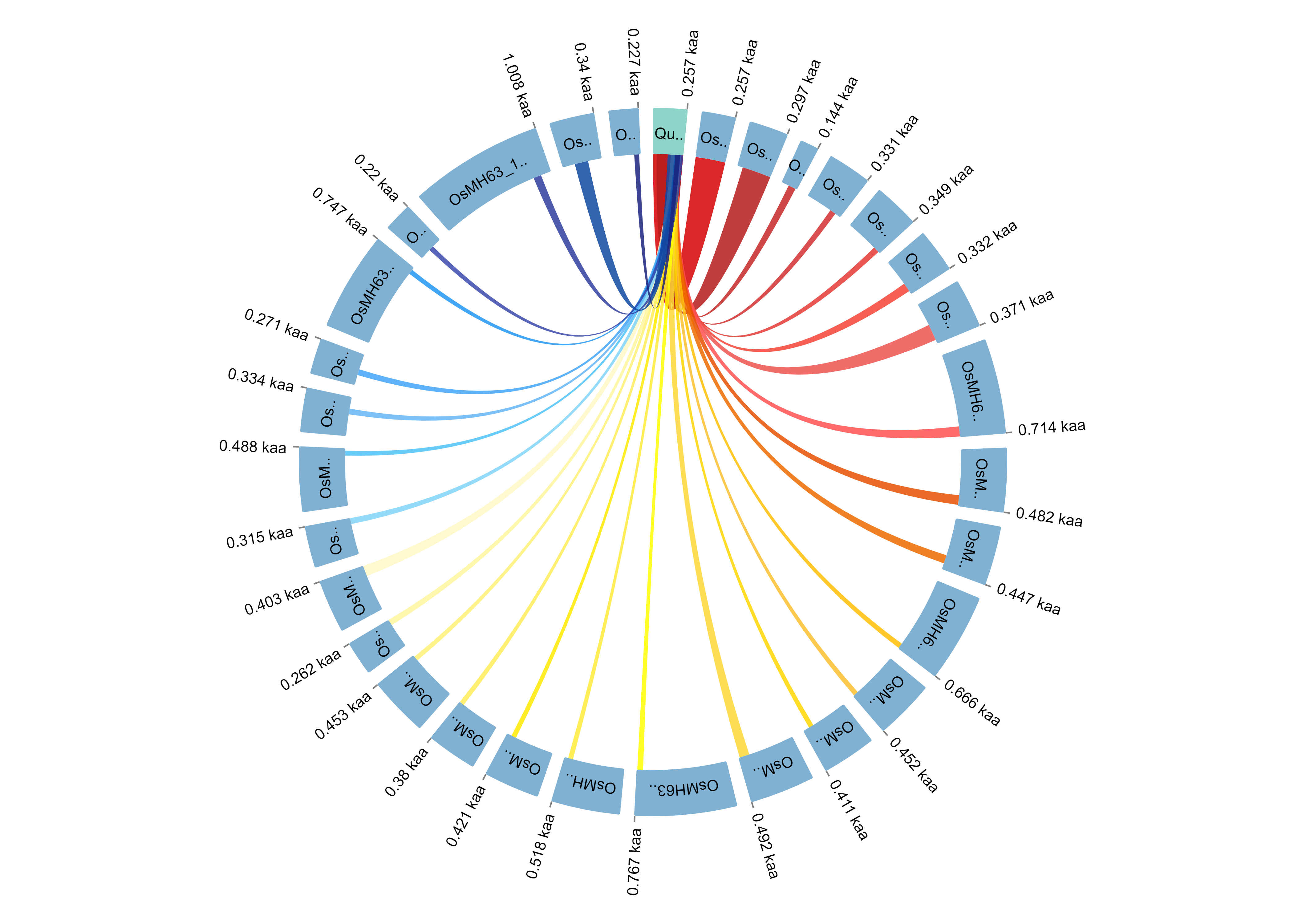
Visualize the results in circle style
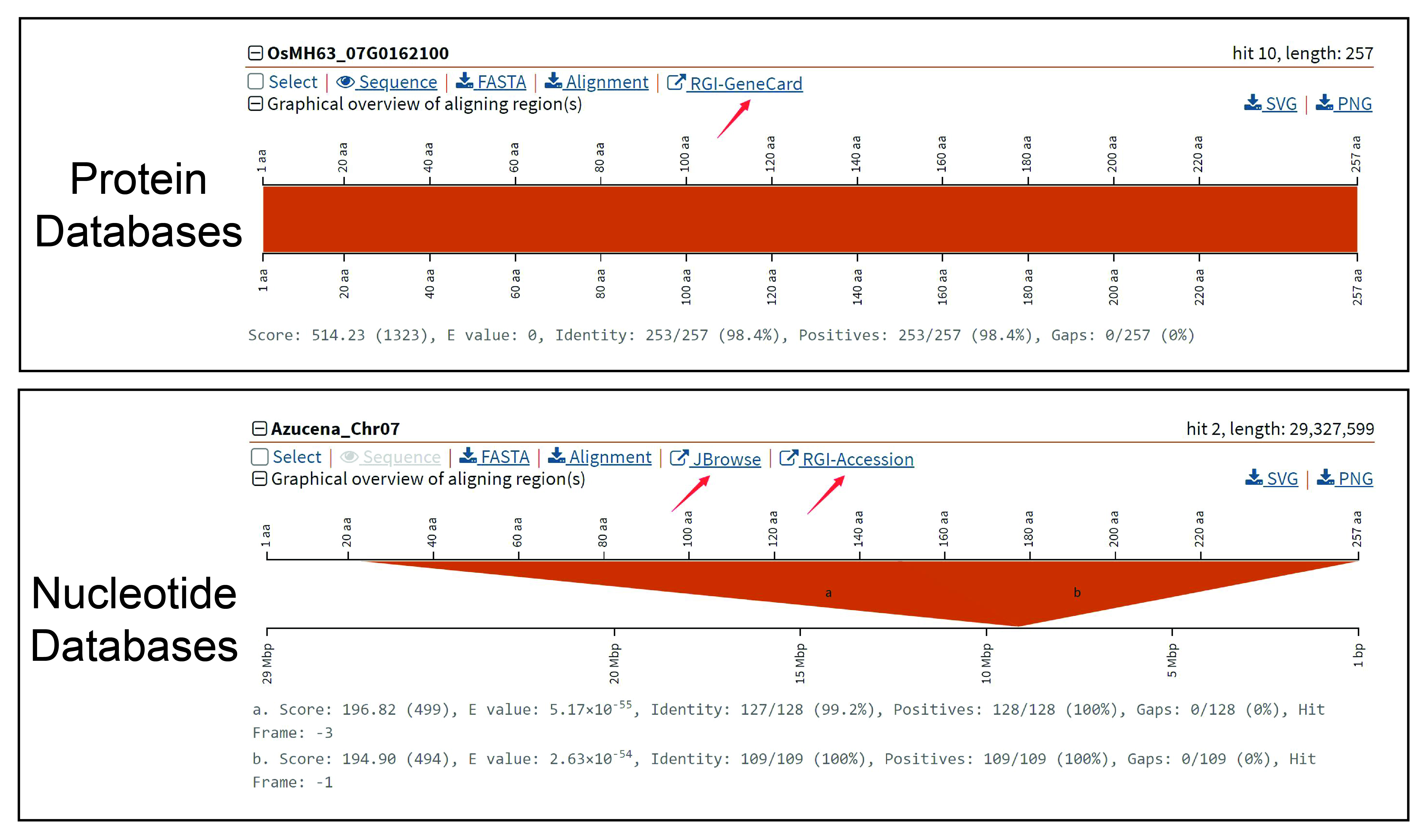
RGI provides match results in text and image formats. Users can easily access the GeneCard of the corresponding gene from the search results based on the protein database, and directly reach the best comparison position on the genome in JBrowse from the search results of the whole genome DNA database. At the same time, the results of the two databases include the sequence, match information, and the download function of block figures.
8. JBrowse

1. The left panel shows tracks that user could be loaded, including protein coding gene annotation, noncoding gene annotation, the RNA-Seq alignment file (cram format) of tissues (leaf, root and panicle) and the transcripts of tissues (leaf, root and panicle) from Iso-Seq data.
2. The main panel shows the structure of genes, transcripts and alignment blocks. User cloud open the pop-up window by click the gene name.
3. The pop-up window shows detailed infromation of gene, and the gene name link to GeneCard module.
9. GOEnrichment
This module provides GO enrichment analysis for users, including single sample GO analysis and multiple samples GO analysis.
9.1. Single sample analysis

1. Select specice you want to search.
2. Select Single sample analysis. Input the foreground gene, such as differential expressed genes, by clipboard or file.
3. (optional) Upload a file (newline splited) containing the background gene list, such as all expressed genes (all genes are used by default).
4. (optional) Set parameters to filter low-confidence GO term (default paramters are Significance value: 0.05, Multi-test adjustment: BH, Min size of genes in background: 5, Max size of genes in background: 1200).
5. Run GOEnrichment module.
6. Download the table of results to .csv file.
7. results. The results show GO term, description, ratio in foreground list, ratio in background, P-value, FDR, number of foreground list, group and gene ID.
Plots

User could visualize the GO enrichment results after get the table of result.
1. Select GO froup (biological procress, cellular component and molecular function).
2. Select visualization style (lollipop, bar, bubble and networks)
3. Plot image.
4. results. It shows the images in four style. The GO terms are grouped by GO group and sorted by -log10(FDR) or ratio.
5. 6. Download the image. User cloud choose figure format and size.
9.2. Multiple samples analysis
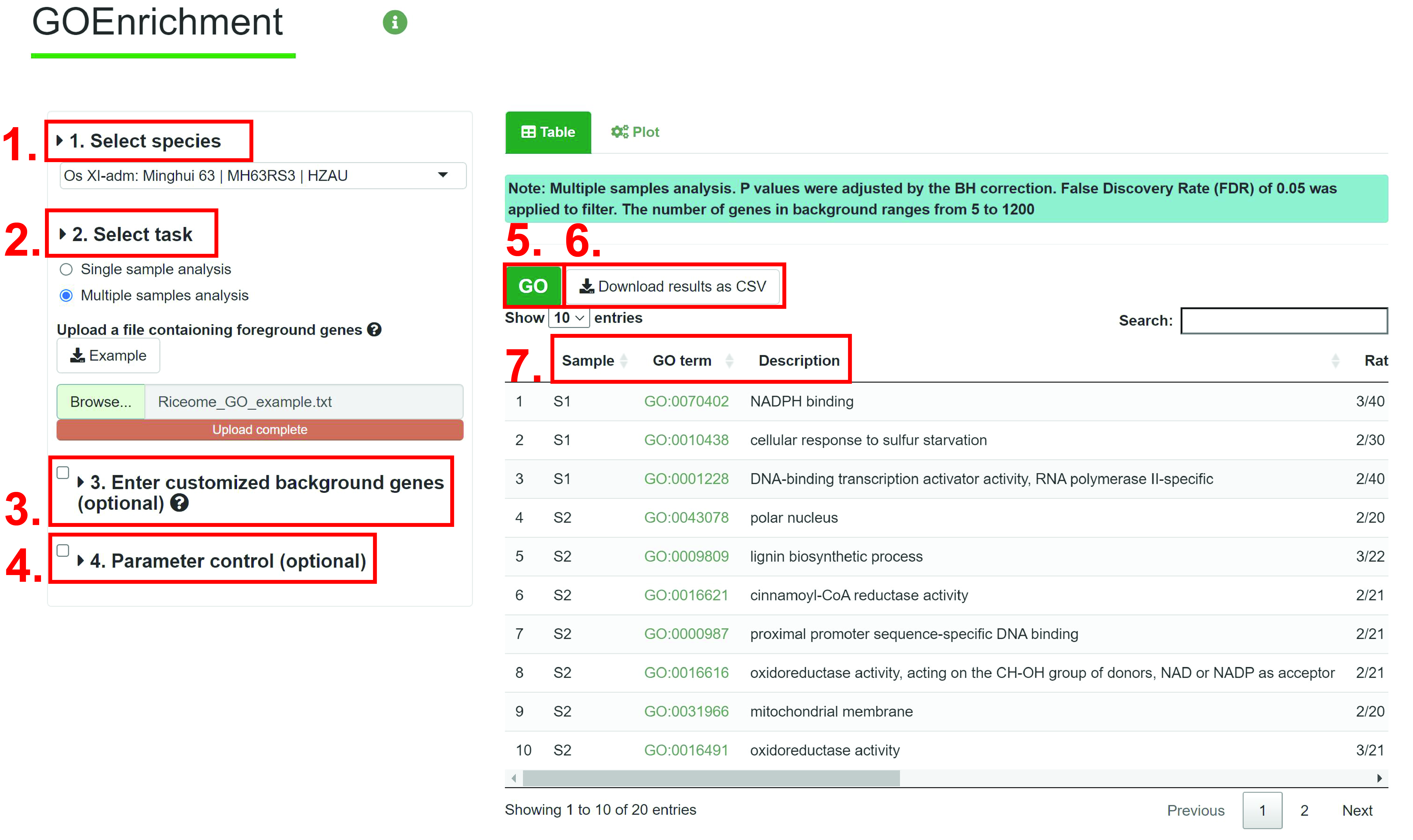
1. Select specice you want to search.
2. Input the foreground gene, such as differential expressed genes (DEGs). The example of input file can be downloaded by clicking the example button.The input file is as follows:
3. (optional) Same as Single sample analysis.
4. (optional) Same as Single sample analysis.
5. Run GOEnrichment module.
6. Download the table of results to .csv file.
7. results. The results show GO term, description, ratio in foreground list, ratio in background, P-value, FDR, number of foreground list, group and gene ID.
Plots
1. Select GO froup (biological procress, cellular component and molecular function).
2. Select samlpes to plot.
3. Plot image.
4. Download the image. User cloud choose figure format and size.
5. results. Each column represents a sample, and each row represents a GO term. The darker the color of the block, the more significant the enrichment result. The GO terms are sorted by -log10(FDR). If the result is not enriched, the color is white.
10. GeneDescription

GeneDescription shows gene location and Description by gene set.
1. Select assembly you want to search.
2. Input gene list by clipboard or file.
3. Run GeneDescription module.
4. Download the table of results to .csv file.
5. results. The results show gene ID, gene location and gene function. And the gene ID column is link to GeneCard to show the comprehensive information.
How to cite RGI
Yu Z, Chen Y, Zhou Y, Zhang Y, Li M, Ouyang Y, Chebotarov D, Mauleon R, Zhao H, Xie W, McNally K, Wing R, Guo W and Zhang J. Rice Gene Index: A comprehensive pan-genome database for comparative and functional genomics of Asian rice. Molecular Plant, 2023, 16(5):798-801. DOI: 10.1016/j.molp.2023.03.012